---

About

ML4Chem is a package to deploy machine learning for chemistry and materials science. It is written in Python 3, and intends to offer modern and rich features to perform machine learning (ML) workflows for chemical physics.

A list of features and ML algorithms are shown below.

• PyTorch backend.

• Completely modular. You can use any part of this package in your project.

• Free software <3. No secrets! Pull requests and additions are more than welcome!

• Documentation (work in progress).

• Explicit and idiomatic: ml4chem.get_me_a_coffee().

• Distributed training in a data parallel paradigm aka mini-batches.

• Scalability and distributed computations are powered by Dask.

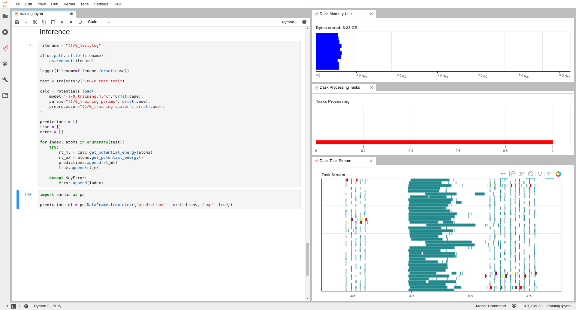
• Real-time tools to track status of your computations.

• Messagepack serialization.

Citing

If you find this software useful, please use this DOI to cite it:

DOI: 10.5281/zenodo.3471761

Documentation

To get started, read the documentation at https://ml4chem.dev. It is arranged in a way that you can go through the theory as well as some code snippets to understand how to use this software. Additionally, you can dive through the module index to get more information about different classes and functions of ML4Chem.

Visualizations

Note: This package is under development.

Copyright

ML4Chem: Machine Learning for Chemistry and Materials (ML4Chem) Copyright (c) 2019, The Regents of the University of California, through Lawrence Berkeley National Laboratory (subject to receipt of any required approvals from the U.S. Dept. of Energy). All rights reserved.

If you have questions about your rights to use or distribute this software, please contact Berkeley Lab’s Intellectual Property Office at IPO@lbl.gov.

NOTICE. This Software was developed under funding from the U.S. Department of Energy and the U.S. Government consequently retains certain rights. As such, the U.S. Government has been granted for itself and others acting on its behalf a paid-up, nonexclusive, irrevocable, worldwide license in the Software to reproduce, distribute copies to the public, prepare derivative works, and perform publicly and display publicly, and to permit other to do so.

Install ML4Chem

You can install ML4Chem from pip, conda or sources.

Pip

You can install ML4Chem and all its dependencies with pip:

python3 -m pip install "ml4chem"

If you want to install the application for your user:

pyhon3 -m pip install --user ml4chem

If you want to install the development version of the master branch:

python3 -m pip install --upgrade git+https://github.com/muammar/ml4chem.git

Conda

For conda installation, execute:

conda install ml4chem

Sources

This type of installation is useful if you are going to develop new features for ML4chem.

1. Clone the application:

   git clone https://github.com/muammar/ml4chem
   

2. Install the requirements:

   cd ml4chem
   python3 -m pip install -r requirements.txt
   

3. After requirements are installed, you can proceed to add ml4chem to your PYTHONPATH and PATH (to use the ml4chem command line tool). Add the following to your .bashrc or .zshrc:

   PYTHOPATH=/path/to/ml4chem:$PYTHONPATH
   PATH=/path/to/ml4chem/bin:$PATH
   

License

ML4Chem: Machine Learning for Chemistry and Materials (ML4Chem) Copyright (c) 2019, The Regents of the University of California, through Lawrence Berkeley National Laboratory (subject to receipt of any required approvals from the U.S. Dept. of Energy). All rights reserved.

Redistribution and use in source and binary forms, with or without modification, are permitted provided that the following conditions are met:

(1) Redistributions of source code must retain the above copyright notice, this list of conditions and the following disclaimer.

(2) Redistributions in binary form must reproduce the above copyright notice, this list of conditions and the following disclaimer in the documentation and/or other materials provided with the distribution.

(3) Neither the name of the University of California, Lawrence Berkeley National Laboratory, U.S. Dept. of Energy nor the names of its contributors may be used to endorse or promote products derived from this software without specific prior written permission.

THIS SOFTWARE IS PROVIDED BY THE COPYRIGHT HOLDERS AND CONTRIBUTORS “AS IS” AND ANY EXPRESS OR IMPLIED WARRANTIES, INCLUDING, BUT NOT LIMITED TO, THE IMPLIED WARRANTIES OF MERCHANTABILITY AND FITNESS FOR A PARTICULAR PURPOSE ARE DISCLAIMED. IN NO EVENT SHALL THE COPYRIGHT OWNER OR CONTRIBUTORS BE LIABLE FOR ANY DIRECT, INDIRECT, INCIDENTAL, SPECIAL, EXEMPLARY, OR CONSEQUENTIAL DAMAGES (INCLUDING, BUT NOT LIMITED TO, PROCUREMENT OF SUBSTITUTE GOODS OR SERVICES; LOSS OF USE, DATA, OR PROFITS; OR BUSINESS INTERRUPTION) HOWEVER CAUSED AND ON ANY THEORY OF LIABILITY, WHETHER IN CONTRACT, STRICT LIABILITY, OR TORT (INCLUDING NEGLIGENCE OR OTHERWISE) ARISING IN ANY WAY OUT OF THE USE OF THIS SOFTWARE, EVEN IF ADVISED OF THE POSSIBILITY OF SUCH DAMAGE.

You are under no obligation whatsoever to provide any bug fixes, patches, or upgrades to the features, functionality or performance of the source code (“Enhancements”) to anyone; however, if you choose to make your Enhancements available either publicly, or directly to Lawrence Berkeley National Laboratory, without imposing a separate written license agreement for such Enhancements, then you hereby grant the following license: a non-exclusive, royalty-free perpetual license to install, use, modify, prepare derivative works, incorporate into other computer software, distribute, and sublicense such enhancements or derivative works thereof, in binary and source code form.

Building Documentation

Documentation is a very important part of any project, and in ML4Chem special attention is given to provide a clear documentation.

To locally build the docs you need to execute the makedocs.sh script:

sh makedocs.sh

This will automatically perform the following commands for you:

cd source
sphinx-apidoc -fo . ../../
cd ..
make html

When the Makefile is finished, you can check the documentation in the build/html folder.

Introduction

Data is central in Machine Learning and ML4Chem provides some tools to prepare your Datas. We support the following input formats:

1. Atomic Simulation Environment (ASE).

We will be adding support to other libraries, soon.

Data

The ml4chem.data.handler module allows users to adapt data to the right format to inter-operate with any other module of Ml4Chem.

Its usage is very simple:

from ml4chem.data.handler import Data
from ase.io import Trajectory

images = Trajectory("images.traj")
data_handler = Data(images, purpose="training")
traing_set, targets = data_handler.get_data(purpose="training")

In the example above, an ASE trajectory file is loaded into memory and passed as an argument to instantiate the Data class with purpose="training". The .get_images() class method returns a hashed dictionary with the molecules in images.traj and the targets variable as a list of energies.

For more information please refer to ml4chem.data.handler.

Introduction

The atomistic module is designed to deploy machine learning (ML) models where the atom is the central object. ML potentials and force fields might be the best known cases of atom-centered models. These models are accurate for tasks such as the prediction of energy and atomic forces. They also are powerful because they can generalize to larger molecular as long as the local environments are sampled extensively to cover large domains.

Theory

The basic idea behind atomistic machine learning is to exploit the phenomenon of “locality” and predict molecular or periodic properties as the sum of local contributions:

\[P = \sum_{i=1}^n P_{atom}(R^{local})\]

where \(P_{atom}\) is a functional of atomic positions. In the case the properties are atomic by nature, e.g. atomic forces or atomic charges, there is no need to carry out the sum shown above as the output of the models are atomic.

Atomic Features

ML models require a set of measurable characteristics, properties or information related to the phenomenon that we want to learn. These are known as “features”, and they play a very important role in any ML model. Features need to be relevant, unique, independent, and for our purposes be physics-constrained e.g. rotational and translational invariance.

ML4Chem supports by default Gaussian symmetry functions, and atomic latent features.

Gaussian symmetry functions

In 2007, Behler and Parrinello [Behler2007] introduced a fixed-length feature vector, referred also as “symmetry functions” (SF), to generalize the representation of high-dimensional potential energy surfaces with artificial neural networks and overcome the limitations related to the image-centered models. These SF are atomic feature vectors constructed purely from atomic positions, and their main objective is to define the relevant chemical environment of atoms in a material.

For building these features, we need to define a cutoff function (\(f_c\)) to delimit the effective range of interactions within the domain of a central atom.

\[\begin{split}f_c(r) = \begin{cases} 0.5(1+cos(\pi \frac{r}{R_c})) , & \text{if}\ r \leq R_c, \\ 0 , & \text{if}\ r \geq R_c, \end{cases}\end{split}\]

where \(R_c\) is the cutoff radius (in unit length), and \(r\) is the inter-atomic distance between atoms \(i\) and \(j\). The cutoff function, having Cosine shape, vanishes for inter-atomic separations larger than \(R_c\) whereas it takes a finite value below the cutoff radius. Cutoff functions avoid abrupt changes on feature magnitudes near the boundary by smoothly damping them.

There are different types of SFs to consider when building Behler-Parrinello feature vectors: i) the radial (two-body term) and ii) angular (three-body terms) SFs. The radial SFs account for all interactions of a central atom \(i\) with its nearest neighbors atoms \(j\). It is defined by,

\[\mathbf{G_i^2} = \sum_{j = 1}^{N_{atom}} e^{-\eta(\mathbf{R_{ij}}-R_{s})^2/R_c^2} f_c(R_{ij}),\]

where \(\mathbf{R_{ij}}\) is the euclidean distance between central \(i\) and neighbor \(j\) atoms, \(R_s\) defines the center of the Gaussian, and \(\eta\) is related to its width. Each value in the sum is normalized by the square of the cutoff radius, \(R_c^2\). In practice, one builds a high-dimensional feature vector by choosing different \(\eta\) values.

In addition to the radial SF, it is possible to include triplet many-body interactions within the cutoff radius \(R_c\) through the following angular SFs:

\[\mathbf{G_i^3} = 2^{1-\zeta} \sum_{j, k \neq i} (1 + \lambda cos\theta_{ijk})^{\zeta} e^{-\eta (\mathbf{R_{ij}}^2 + \mathbf{R_{ik}}^2 + \mathbf{R_{jk}}^2)/R_c^2} f_c(R_{ij}) f_c(R_{ik}) f_c(R_{jk}).\]

This part of the features is built from considering the Cosine between all possible \(\theta_{ijk}\) angle of a central atom. There exists a variant of \(\mathbf{G_i^3}\) that includes three-body interactions of atoms forming \(180^{\circ}\) inside the cutoff sphere but having an interatomic separation larger than \(Rc\). These SFs account for long-range interactions [Behler2015]:

\[\mathbf{G_i^4} = 2^{1-\zeta} \sum_{j, k \neq i} (1 + \lambda cos\theta_{ijk})^{\zeta} e^{-\eta (\mathbf{R_{ij}}^2 + \mathbf{R_{ik}}^2)/R_c^2} f_c(R_{ij}) f_c(R_{ik}).\]

An atomic Behler-Parrinello feature vector will be composed by a subvector with radial SFs and another subvector of angular SFs. This represents an advantage when it comes to evaluate which type of SFs is more important when predicting energy and atomic forces.

from ml4chem.atomistic.features.gaussian import Gaussian

features = Gaussian(cutoff=6.5, normalized=True, save_preprocessor="features.scaler")

In the code snippet above we are building Gaussian type features using the ml4chem.atomistic.features.gaussian.Gaussian class. We use a cutoff radius of \(6.5\) angstrom, we normalized by the squared cutoff raidous, and the preprocessing is saved to the file features.scaler (by default the preprocessing used is MinMaxScaler in a range \((-1, 1)\) as implemented in scikit-learn). The angular symmetry functions used by default are \(G_i^3\), if you are interested in using \(G_i^4\), then you need to pass angular_type keyword argument:

features = Gaussian(cutoff=6.5, normalized=True,
                    save_preprocessor="features.scaler", angular_type="G4")

Atomic latent features

These features are decided by the neural network and can be obtained with the Autoencoder class.

Models

Neural Networks

Neural Network (NN) are models inspired on how the human brain works. They consist of a set of hidden-layers with some nodes (neurons). The most simple NN architecture is the fully-connected case in which each neuron is inter-connected to every other neuron in the previous/next layer, and each connection has its own weight. When an activation function is applied to the output of a neuron, the NN is able to learn non-linearity aspects from the data.

In ML4Chem, a neural network can be instantiated as shown below:

from ml4chem.atomistic.models.neuralnetwork import NeuralNetwork

n = 10
activation = "relu"
nn = NeuralNetwork(hiddenlayers=(n, n), activation=activation)
nn.prepare_model()

Here, we are building a NN with the ml4chem.atomistic.models.neuralnetwork.NeuralNetwork class with two hidden-layers composed 10 neurons each, and a ReLu activation function.

Autoencoders

Autoencoders (AE) are NN architectures that able to extract features from data in an unsupervised learning manner. AE learns how to encode information because of a hidden-layer that serves as an informational bottleneck as shown in the figure below. In addition, this latent code is used by the decoder to reconstruct the input data.

from ml4chem.atomistic.models.autoencoders import AutoEncoder

hiddenlayers = {"encoder": (20, 10, 4), "decoder": (4, 10, 20)}
activation = "tanh"
autoencoder = AutoEncoder(hiddenlayers=hiddenlayers, activation=activation)
data_handler.get_unique_element_symbols(images, purpose=purpose)
autoencoder.prepare_model(input_dimension, output_dimension, data=data_handler)

ML4Chem also provides access to variational autoencoders (VAE) [Kingma2013]. These architectures differ from an AE in that the encoder codes a distribution with mean and variance (two vectors with the desired latent space dimension) instead of a single latent vector. Subsequently, this distribution is sampled and used by the decoder to reconstruct the input. This creates a generative model because now we will generate a latent distribution that allows a continuous change from one class to another.

To use this architecture, it just suffices to change the snippet shown above for an AE as follows:

from ml4chem.atomistic.models.autoencoders import VAE

hiddenlayers = {"encoder": (20, 10, 4), "decoder": (4, 10, 20)}
activation = "tanh"
vae = VAE(hiddenlayers=hiddenlayers, activation=activation, variant="multivariate")
data_handler.get_unique_element_symbols(images, purpose=purpose)
vae.prepare_model(input_dimension, output_dimension, data=data_handler)

Kernel Ridge Regression

Kernel Ridge Regression (KRR) is a type of support vector machine model that combines Ridge Regression with the kernel trick. In ML4Chem, this method is implemeted as described by Rupp in Ref. [Rupp2015]. Below there is a description of this implementation:

1. Molecules are featurized.

2. A kernel function \(k(x, y)\) is applied to all possible pairs of atoms in the training data to build a covariance matrix, \(\mathbf{K}\).

3. \(\mathbf{K}\) is decomposed in upper- and lower- triangular matrices using Cholesky decomposition.

4. Finally, forward- and backward substitution is carried out with desired targets.

Gaussian Process Regression

Gaussian Process Regression (GP) is similar to KRR with the addition of the uncertainty of each prediction.

References:

Behler2007

Behler, J. & Parrinello, M. Generalized Neural-Network Representation of High-Dimensional Potential-Energy Surfaces. Phys. Rev. Lett. 98, 146401 (2007).

Behler2015

Behler, J. Constructing high-dimensional neural network potentials: A tutorial review. Int. J. Quantum Chem. 115, 1032–1050 (2015).

Kingma2013

Kingma, D. P. & Welling, M. Auto-Encoding Variational Bayes. arXiv Prepr. arXiv1312.6114 (2013).

Rupp2015

Rupp, M. Machine learning for quantum mechanics in a nutshell. Int. J. Quantum Chem. 115, 1058–1073 (2015).

Visualization

We also offer a ml4chem.visualization module to plot interesting graphics about your model, features, or even monitor the progress of the loss function and error minimization.

Two backends are supported to plot in ML4Chem: Seaborn and Plotly.

An example is shown below:

from ml4chem.visualization import plot_atomic_features
fig = plot_atomic_features("latent_space.db",
                           method="pca",
                           dimensions=3,
                           backend="plotly")
fig.write_html("latent_example.html")

This will produce an interactive plot with plotly where dimensionality was reduced using PCA, and an html with the name latent_example.html is created.

To activate plotly in Jupyter or JupyterLab follow the instructions shown in https://plot.ly/python/getting-started/#jupyter-notebook-support

If plotly is not rendering correctly you need to install the jupyter extension:

jupyter labextension install @jupyterlab/plotly-extension

Indices and tables

• Index

• Module Index

• Search Page